
Going about doctoral thesis writing, love hate relationship, the thought occurred to me perhaps the very field I’m writing on about has already lived past its Golden Era, or has it?
A knee jerk reaction then was to see if there’s any python or R package which allows me to search the abstracts with the keyword microbiome… this turned up pubmed_parser. However, in order to get this running, I will have to first download a few gigabytes of abstracts in XML from the Open Access subset of pubmed abstracts and run my own pyspark…
NOPE! Not going there!
Then it occurred to me perhaps NCBI has something I could use… in the previous post we talked about the esearch API. Hmmm, this could be useful.
So below’s the script which lets me do this:
Libraries
using the usual tidyverse, with rvest for XML parsing and artyfarty to spruce up the plot
suppressPackageStartupMessages({
    library(tidyverse)
    library(magrittr)
    library(rvest) # for XML
    library(artyfarty) #because theme_bw is too boring
})
NCBI ESEARCH
Here’s the NBCI’s esearch API. Within it, there’s the date range options, mindate, maxdate.
mindate, maxdate API filter
Date range used to limit a search result by the date specified by datetype. These two parameters (mindate, maxdate) must be used together to specify an arbitrary date range. The general date format is YYYY/MM/DD, and these variants are also allowed: YYYY, YYYY/MM.
So we will be searching between 1997 to 2017, a 20 year period.
So lets begin …..
Keyword: Microbiome
with other synonyms microbiota
#microbiome
api="https://eutils.ncbi.nlm.nih.gov/entrez/eutils/esearch.fcgi?"
query="db=pubmed&term=%s&mindate=%s&maxdate=%s"
searchTerm=paste0(api, query)

keyword = "microbiome"

df = mapply(function(start, end){
            count = read_xml(sprintf(searchTerm, keyword, start, end)) %>%
            as_list %$%
            Count %>%
            unlist
       tibble(count, start, end)
},  start = 1997:2016,
    end = 1998:2017,
    SIMPLIFY=FALSE
) %>% do.call(rbind,.)
Keyword: Cancer
Used as a comparison
keyword = "cancer"

df2 = mapply(function(start, end){
            count = read_xml(sprintf(searchTerm, keyword, start, end)) %>%
            as_list %$%
            Count %>%
            unlist
       tibble(count, start, end)
},  start = 1997:2016,
    end = 1998:2017,
    SIMPLIFY=FALSE
) %>% do.call(rbind,.)
Putting the two together before we start plotting
df %<>% setNames(c("microbiome", "start", "end"))
df %<>% mutate(cancer = as.integer(df2$count))
df$microbiome %<>% as.integer
df %<>% select(start, end, microbiome, cancer)
df
As you can the see the order is slighly different between the two, you’ll probably have to do some scaling.
| start | end | microbiome | cancer |
|---|---|---|---|
| 1997 | 1998 | 91 | 116522 |
| 1998 | 1999 | 110 | 124613 |
| 1999 | 2000 | 133 | 131481 |
| 2000 | 2001 | 149 | 139577 |
| 2001 | 2002 | 196 | 153651 |
| 2002 | 2003 | 249 | 166393 |
| 2003 | 2004 | 304 | 170676 |
| 2004 | 2005 | 419 | 181504 |
| 2005 | 2006 | 576 | 190710 |
| 2006 | 2007 | 744 | 198618 |
| 2007 | 2008 | 955 | 210488 |
| 2008 | 2009 | 1285 | 219686 |
| 2009 | 2010 | 1741 | 231079 |
| 2010 | 2011 | 2610 | 248046 |
| 2011 | 2012 | 3899 | 265171 |
| 2012 | 2013 | 5607 | 281240 |
| 2013 | 2014 | 8211 | 308483 |
| 2014 | 2015 | 10951 | 331775 |
| 2015 | 2016 | 13439 | 331631 |
| 2016 | 2017 | 14058 | 285408 |
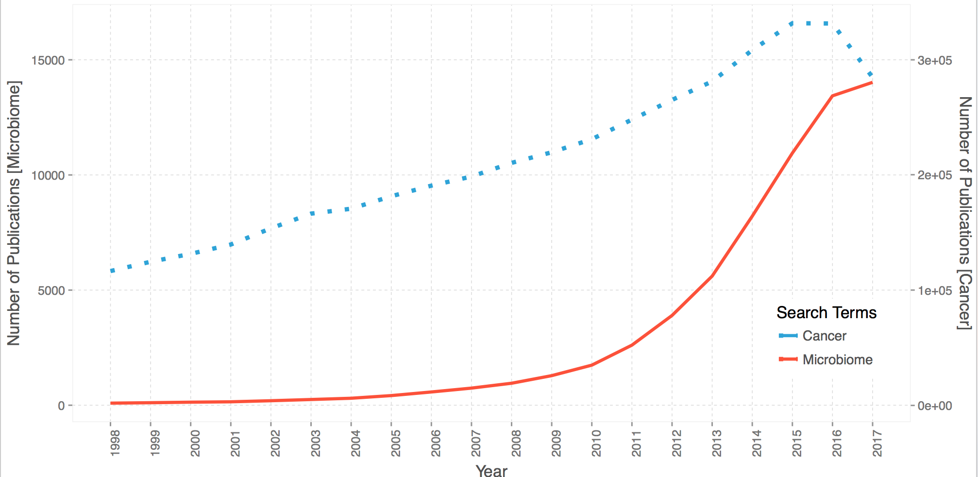
Since version 2.2.0 of ggplot2, Hadley has included the sec_axis function in the library which lets you add a secondary axis as long as it’s amenable to a straight forward transformation.
ggplot(df, aes(x=end)) +
    geom_line(aes(y=microbiome, color="Microbiome"), size=1.1) +
    geom_line(aes(y=cancer/20, color="Cancer"), size=1.5, linetype="dotted") +
    # manipulated the cancer values by dividing by 20
    scale_x_continuous(breaks=1998:2017)+
    scale_y_continuous(sec.axis = sec_axis(~.*20, name = "Number of Publications [Cancer]"))+
    # restores the division
    # lets we set the axis title
    scale_color_manual("Search Terms",values = pal("five38"))+
    theme_scientific() +
    theme(axis.text.x=element_text(angle=90),
          legend.position = c(0.9, 0.2)) +
    xlab("Year") + ylab("Number of Publications [Microbiome]")
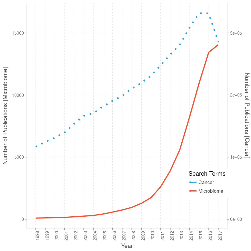
There you have it guys, on the left y-axis the publication count with the keyword “microbiome” and its synonyms like “microbiota” and on the right y-axis the counts for abstract with the keyword “cancer”. As you can see, the growth in publications/articles revolving around microbiome or at least associated to it have been growing at breakneck pace faster than cancer, almost exponential.
For those astute enought, you’ll notice a dip in 2017 for cancer, and the trend is slowing down for microbiome, that’s just cause we haven’t reached the end of 2017 yet, close 😉 but definitely more papers on their way.
Hope this will be helpful for future students! Cheers
comments powered by Disqus