Introduction

Since our earlier post, I’ve defended my thesis, moved on from Honestbee to AirAsia to work on dynamic/auto base pricing Ancillary products. However COVID-19 happened and I found myself in the ride hailing GrabTransport / deliveries GrabFood industry again. Time does pass by quickly.

The following post does not represent my employer and reflects my own personal views only.

Once again, spark makes a return in my current job. After using Redshift and GCP’s BigQuery, I’ve formed myself a working style which separates ETL work for example feature engineering in SQL and model training at first in a notebook then formalised as a class object and finally a script or ML pipeline.

In my opinion, SQL as king since it is the common tongue amongst data practitioners: Engineers, Scientists and Analysts.

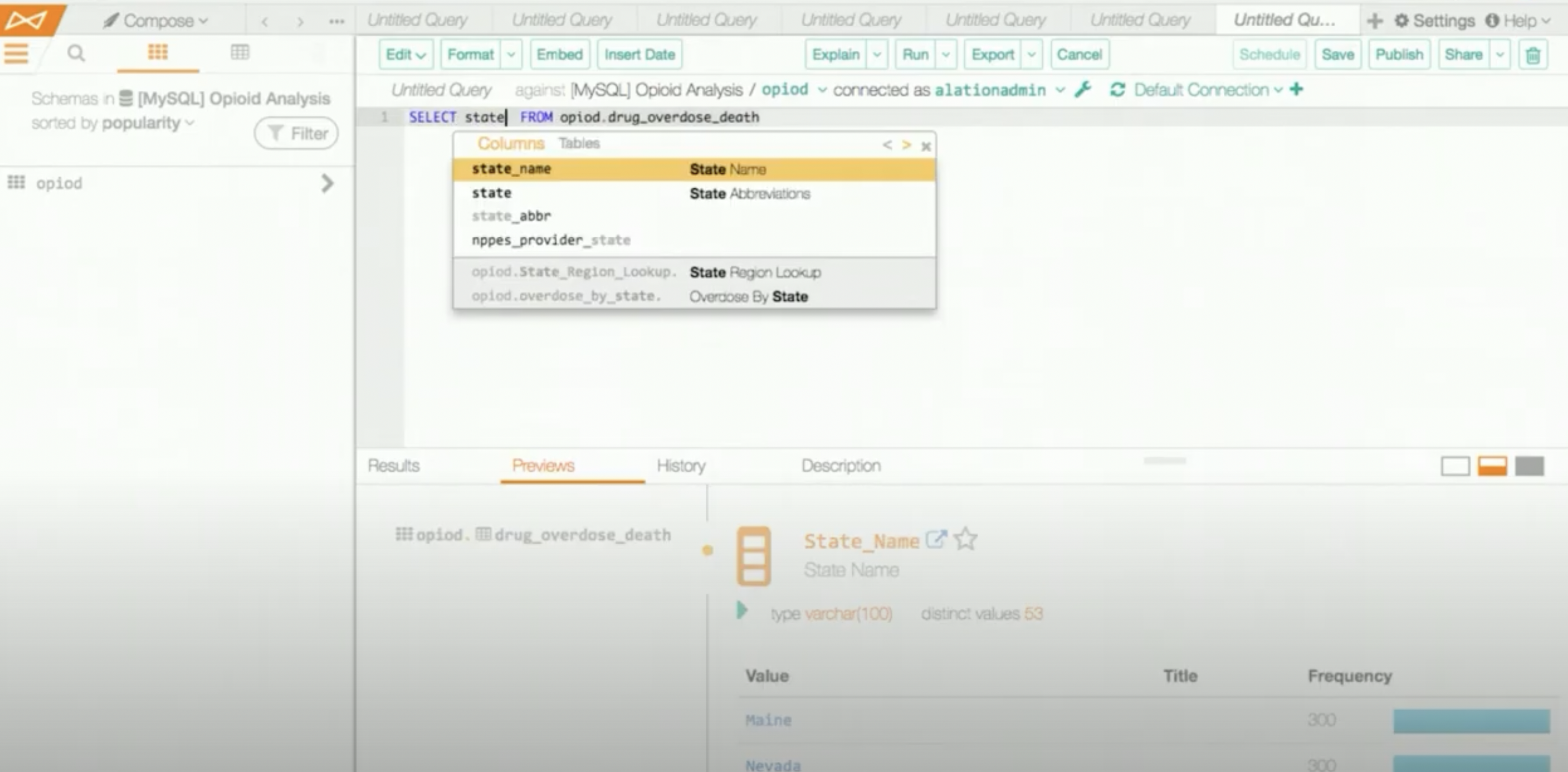
As for the ETL portion, nothing too drastic has changed. For quick and dirty data exploration I would use the web SQL workbench offered by Alation Compose the web-based editor offered by the company’s official data catalog and does not require one to set up any login credentials with a local client like DataGrip or DBeaver. Both BigQuery and Alation (presto) offers the ability to share queries via a link and has excellent access control. Important information about tables are also found in the catalog ie. column descriptions, PII, data owner and is very similar to the features offered by GCP’s data catalog.

However, this time, instead of Redshift or Bigquery there is HIVE. tables exists within the Hive MetaStore (HMS) which I struggled to learn how to add drop tables to with initially. Also there was a decoupling of the query engine with the data warehouse was quite jarring at first since there were two dialects used by the company, spark SQL and Presto SQL. With bigquery the query engine is part of the datawarehouse.

This succinct decoupling of (1) storage, (2) query engine and (3) metastore was quite new to me. It was only later after doing some reading on my own, that I was able to map BigQuery to the current setup. For example, instead of colossus there is S3 for my file system. And for the query engine instead of dremel you would have a constantly available presto cluster or a transient spark cluster to do heavier lifting jobs. Table and metadata are stored in HIVE MetaStore (HMS).

Only when I need to carry out some in-depth analysis / feature engineering + model building. Previously in Honestbee we used an external vendor to maintain our spark infrastructure while in the current company, we have a in-house team managing the spark clusters to be cost efficient. Similar to BQ’s datasets and tables, we are able to save tables in HMS. However this was not very clear initially and this post aims to bridge any knowledge gaps using Spark as the query engine, I might decide to include a edit or new post of using Presto to build views in HIVE.

SparkSession

Sadly the companies I’ve worked in are mostly python centric and the use of R has also decreased. However I still use GGPLOT2 for plotting although there has been more some developments porting it to python.

Similar to R’s sparklyr package we create a spark connection of type SparkSession (it is often aliased as spark) in PySpark

Since spark 2.X, Spark Session unifies the Spark Context and Hive Context classes into a single interface. Its use is recommended over the older APIs for code targeting Spark 2.0.0 and above.

InputOutput

With HIVE support enabled, spark queries can query against tables found in HMS whose partitions are known beforehand or directly against files stored in buckets, if they are not registered in HMS.

Input

Spark supports querying against a metastore like a traditional data warehouse but you can also query against flat files in S3. Like how you can create tables in BQ with external files eg. CSV or parquet.

External files

A common format is parquet, you could register the data as a table in HMS or just work on it in memory. If you do not need register this as a table you can read the files directly into memory like the following.

You’ll be able to register this as a in-memory view using df.createTempView("<view_name">) and you might also consider caching to load the whole table into memory. Since this DataFrame only exists in memory and it’s not registered in HMS there’s no table partition. However the in-memory RDDs are partitioned.

Output

If you would like the results of the ETL/query to persist so you can query it again later sometime in the future, you could save the results as an intermediate step which is archived or for machine learning either in parquet or Tensorflow’s TFRecord format.

Tensorflow

The recommended file format is tf.Data.TFRecordDataset when working with Tensorflow framework.

You can save your results to this format using the following (gzipped to save space)

💡 To use the tfrecords format, remember to include the connector JAR and place it in the extra_classpath. At the point of writing org.tensorflow:spark-tensorflow-connector_2.11:1.115 works with the Gzip codec

Registering tables in HMS with parquet files in S3

Similar to how BigQuery stores the underlying data of tables in capacitor , columnar file format stored in google’s file system colossus. (GCS is built on top of colossus). It’s recommend to store the data in parquet also a columnar file format in S3.

TIP: The fastest way to check if the table exists is to run DESCRIBE schema.table

In the following example we are going to assume that the parquet files are stored in the following path: s3://datascience-bucket/wesley.goi/data/pricing/demand_tbl/

Partitioned tables in HMS

When working with spark and HMS, one has to be mindful of the term partition, In spark, the term refers to data partitioning in Resilient Distributed Datasets (RDD), where partitions represent chunks of data sent to workers/executors for parallel processing. In HMS, the term represents how the data is stored in the cloud file system eg. S3 and helps guide queries agains the dataset in an efficient manner which is closer to the partitioned tables in databases.

First you’ll need to be able to save the data in S3, there’s a specific naming conversion for the file path which you’ll need to follow ie. s3://<bucket>/prefix/key=value.

As you have seen, one of the most common ways to partition a table is via timestamp eg. s3://<bucket>/prefix/date=YYYYMMDD

One can also partition on multiple columns although in a nested manner eg. folder/year=2021/month=03/day=21

Where the folder structure follows:

Year=yyyy
 |---Month=mm
 |   |---Day=dd
 |   |   |---<parquet-files>

⚠️: Check if the external table which you’re querying is already partitioned. SHOW PARTITIONS table

💡You can check the number of partitions scanned if you run .explain(mode="formatted") to see

Generate Column data type schema

Manual

You can prepare the table column schema like BigQuery manually and save it in a JSON file and parse it.

Infer

Create table

To create a table in HIVE, we will be using the CREATE statement from HIVE SQL.

You might also want to check if the table exists:

Insert partitions

In this example we will be adding s3://datascience-bucket/wesley.goi/data/pricing/demand_tbl/year=2021/month=01/day=11/hour=01

You can check if the partition has been add by running SHOW PARTITIONS pricing.demand_tbl

However when you query the table you’ll notice that you cannot query the partition yet.

You’ll still have to refresh the table for that partition

Remember to refresh

Bulk import

If you have multiple partitions and do not wish to rerun the above for each partition, you may wish to run the MSCK command to sync the all files to the HMS.

Temp Views / Tables

In the same spark session, it is possible to create a temp view. Temp views should not be confused with views in BigQuery, these are not registered in HMS and persists only for the duration of the given SparkSession.

Data is stored in memory in-memory columnar format.

These are especially useful if the data manipulation is complicated and multi stepped and you wish to persist some intermediate tables. In BQ, I would just save temp as a table.

NOTE: temp tables == temp views.

From a query:

Views

Unfortunately you cannot register a view in HIVE using spark but you can do so in presto.

Sampling

Often when training your model, you might need to sample from the existing dataset due to memory constraints.

You might want to set a seed as well when caching if you are doing hyperparameter tuning so you will get the same dataset on each iteration. And set the withReplacement parameter to be False.

Caching

Caching is not lazy with ANSI SQL, and it will be stored in memory immediately.

Compared to PySpark df.cache() (you’ll have to run df.count() to force the table to be loaded into memory), the above SQL statement is not lazy and will store the table in memory once executed.

UDFs

User-Defined-Functions (UDFs) are ways to define your own functions. Which you can write in python before declaring it for use in SQL using spark.udf.register

NOTE: If UDF requires C binaries which needs to be compiled, you’ll need to install in the image used by the worker nodes.

SQL Hints

Hints go way back as early as spark 2.2, which introduced. These could be grouped into several categories.

Repartitioning

By default when repartitioning, it’ll be set to 200 partitions, you might not want this and to optimise the query you might want to hint spark otherwise

1. REPARTITION
2. COALESCE only reduces the number of partitions, optimised version of repartition. Data which is kept on the original nodes and only those which needs to be moved are moved (see example below)
3. REPARTITION_BY_RANGE eg. You have records which has a running id from 0 - 100000 and you’ll want to split them into 3 partitions repartitionByRange(col, 3)

When coalescing you’re shrinking the number of nodes on which the data is kept eg. From 4 to

# original
Node 1 = 1,2,3
Node 2 = 4,5,6
Node 3 = 7,8,9
Node 4 = 10,11,12

# Coalescing from 4 to 2 partitions:
Node 1 = 1,2,3 + (10,11,12)
Node 3 = 7,8,9 + (4,5,6)

You can also improve query time by including columns when repartitioning especially if you are joining on these columns. This applies to tables as well as temp views.

You can also chain multiple repartition hints: repartition(100), coalesce(500) and repartition by range for column c into 3 partitions

https://spark.apache.org/docs/3.0.0/sql-ref-syntax-qry-select-hints.html the optimised plan is as follows:

# Repartition to 100 partitions with respect to column c.
== Optimized Logical Plan ==
Repartition 100, true
+- Relation[name#29,c#30] parquet

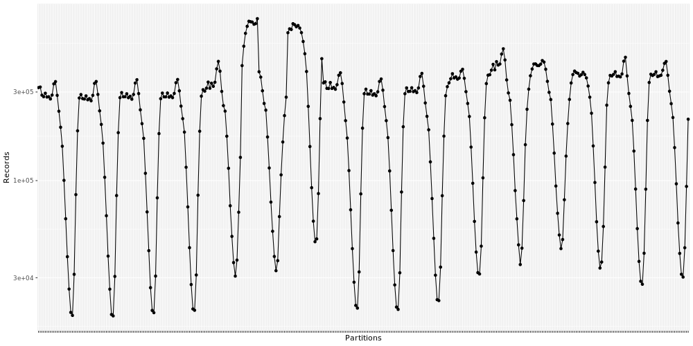
Often the number of records per partition is not equal, especially if you’re partitioning by time and you might end up the number of records per partition following a cyclic pattern. eg. Traffic at night is much lesser than traffic in the day.

Join hints

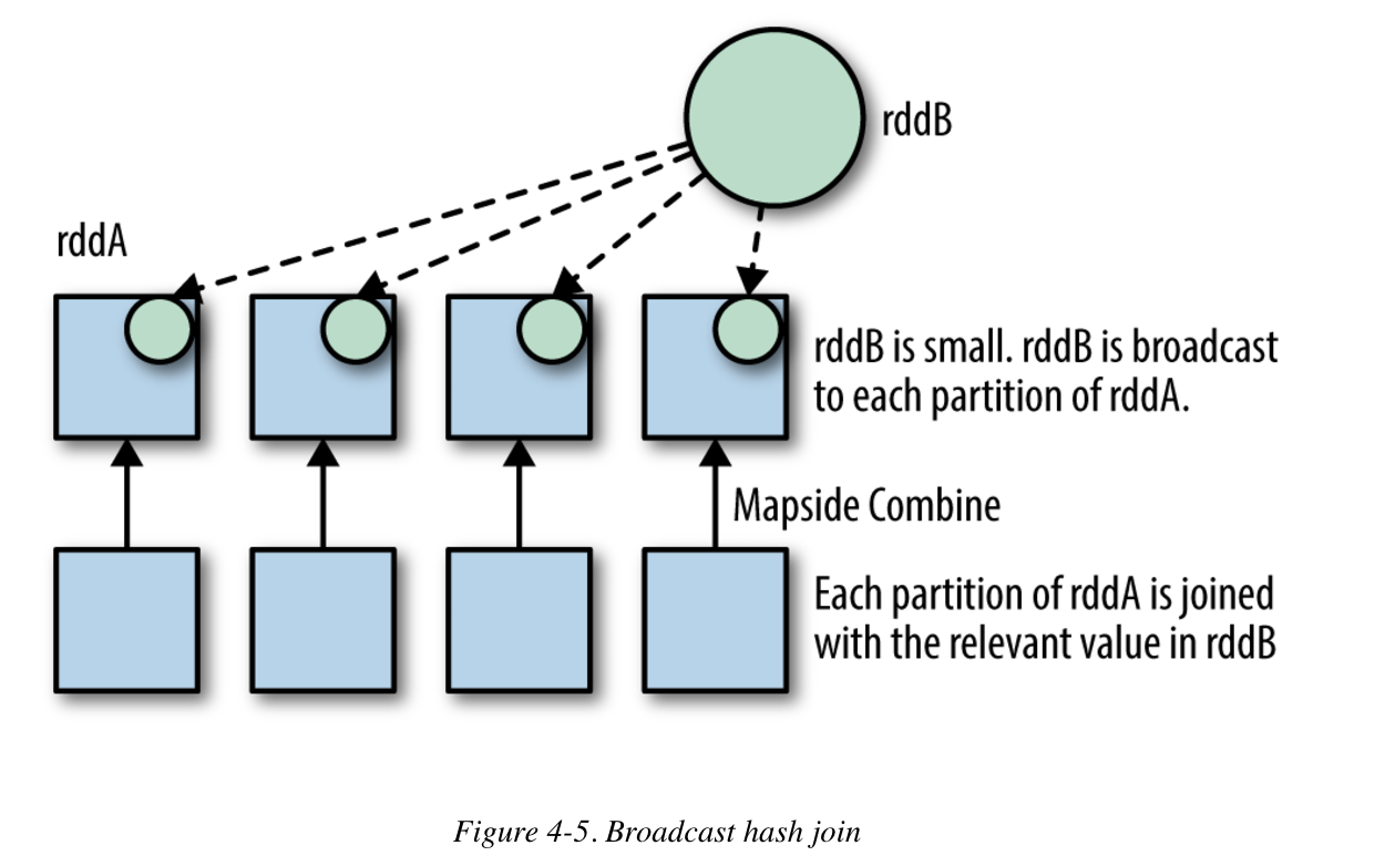
• BROADCAST JOIN replicates the full dataset (if it can fit into memory of the workers) into all nodes

These are useful for selective joins (where the output is expected to small), when memory is not an issue and it’s the right table in a left join.

• MERGE : shuffle sort merge join
• SHUFFLE_HASH: shuffle hash join. If both sides have the shuffle hash hints, Spark chooses the smaller side (based on stats) as the build side.
• SHUFFLE_REPLICATE_NL: shuffle-and-replicate nested loop join

Adaptive Query Execution (AQE)

Another new feature which comes with spark3 is the AQE. Previously the query plan is done prior to execution and no optimisation is done thereafter.

Partitions

One of the areas which sets itself up for optimisation during execution is the to determine the optimum number of partitions. By default,spark.sql.shuffle.partitions is set to 200, in cases when the dataset is small, this number would be too large while the reverse is also true.

Broadcast Joins

If the table from any side is smaller than broadcast in in hash join threshold, sort merge joins are automatically converted to a broadcast join.

You can try this AQE Demo - Databricks

CustomShuffleReader indicates it’s using AQE and it ends with AdaptiveSparkPlan